Jupyter (Colaboratory) Notebooks

This tutorial was inspired by and adapted from Shawn A. Rhoads’ PSYC 347 Course [CC BY-SA 4.0 License] and Jeremy Manning’s PSYC 32 Course [MIT License].

Learning objectives

This notebook is intended to teach you:

1. How to set up your Google Colaboratory

2. How to use Jupyter (Colaboratory) notebooks

Setting up your Google Colaboratory Account

Google Colaboratory

Google Colaboratory is a system for writing and running code through a web browser. Your files are stored on Google Drive, and code that you run is executed on a remote Google Cloud server. To learn more about Google Colaboratory, check out this document.

Google Colaboratory (including access to Google Cloud computers) is included as part of all Google accounts. To gain access to this resource, you first need to sign up for a Google account (if you don’t already have one). Remember your username (email address) and password; you’ll use it throughout the term and you’ll rely on Colaboratory for most of your slides.

You can sign up for a Google account here. Once you’ve signed into your Google account, you can access Google Colaboratory here.

How to use Jupyter (Colaboratory) notebooks

The document you’re viewing right now is a Jupyter notebook. A Jupyter notebook is a file (extension: .ipynb, which stands for “interactive Python notebook). The contents of Jupyter notebooks are stored as .json (JavaScript Object Notation) files. It’s not super important that you familiarize yourself with the nitty-gritties of the .json format at the moment.

What’s a Jupyter notebook?

From Jupyer Notebook: An Introduction

The Jupyter Notebook is an open source web application that you can use to create and share documents that contain live code, equations, visualizations, and text. Jupyter Notebook is maintained by the people at Project Jupyter.

Jupyter Notebooks are a spin-off project from the IPython project, which used to have an IPython Notebook project itself. The name, Jupyter, comes from the core supported programming languages that it supports: Julia, Python, and R. Jupyter ships with the IPython kernel, which allows you to write your programs in Python, but there are currently over 100 other kernels that you can also use.

For a more complete answer, check out this video. The short answer is that a Jupyter notebook is an interactive tool that allows you to take notes, execute code, create figures, and easily share it all with other people. Jupyter notebooks comprise a series of cells. Each cell (looks like a rectangular block of text) in a notebook contains one of two basic categories of content:

We will use Jupyter Notebooks to interface with Python. Rather than keeping code scripts code and execution separate, Jupyter integrates both together using the concept of cells. Two main types of cells are code cells and markdown cells. Cells pair “snippets” of code with the output obtained from running them and can contain plots/figures inline alongside code required to generate them.

Interactive Coding!!

Code cells

Markdown cells

Code cells contain actual code that you want to run. You can specify a cell as a code cell using the pulldown menu in the toolbar in your Jupyter notebook. Otherwise, you can hit esc and then y (denoted “esc, y”) while a cell is selected to specify that it is a code cell. Note that you will have to hit enter after doing this to start editing it. If you want to execute the code in a code cell, hit “shift + enter”. Note that code cells are executed in the order you execute them. That is to say, the ordering of the cells for which you hit “shift + enter” is the order in which the code is executed. If you did not explicitly execute a cell early in the document, its results are now known to the Python interpreter.

Markdown cells (like the current cell) contain formatted text in the Markdown text formatting language. You can read about its syntax here. You can use these cells kind of like the code underlying text you’d write in a word processor. For the most part, text in Markdown cells gets “rendered” (i.e. drawn on the screen) just as you write it. However, you can also specify various formatting tweaks, like creating italicized or bolded text, etc. This tutorial provides a quick and gentle interactive introduction to Markdown. You can create a new Markdown cell by pressing the “+” button in the toolbar and selecting “Markdown” from the dropdown list in the toolbar. Note that you can also insert HTML into markdown cells, and this will be rendered properly. Hitting “shift + enter” renders the text in the formatting you specify. You can specify a cell as being a markdown cell in the Jupyter toolbar, or by hitting “esc, m” in the cell. Again, you have to hit enter after using the quick keys to bring the cell into edit mode.

In general, when you want to add a new cell, you can use the “Insert” pulldown menu from the Jupyter toolbar. The shortcut to insert a cell below is “esc, b” and to insert a cell above is “esc, a”. Alternatively, you can execute a cell and automatically add a new one below it by hitting “alt + enter”.

The text you type into a new notebook cell is a set of instructions that tell the notebook what to do when the cell is run (i.e., transformed from a set of instructions into an executed set of actions). To run a cell, hold the shift key and press enter/return.

• When you run a Markdown cell, the text is rendered with the formatting options you specify. To see and/or edit the underlying code, simply double click on the rendered text.

• When you run a Code cell, the Python instructions you type in are run. We’ll explore what this means below. Note: the first time you run a Code cell in Google Colaboratory, you’ll see a warning message pop up (asking if it’s okay to run code not authored by Google). You should give the notebook permission to run so that you can interact with it.

Running Python code in Jupyter notebooks

If you’re accessing this notebook within Google Colaboratory, you can interact with Code by running it on Google’s computers (via Google Cloud– i.e., Google’s high performance computing cluster). The first time you run a command within a colaboratory notebook, you’ll automatically be allocated a virtual computer (i.e., a simulation of a computer that’s running somewhere on Google’s servers). It takes a few seconds to boot that system up (you’ll see a “connecting” message in the upper right when the new computer is being allocated, and you’ll see a bar graph showing RAM and disk usage once the computer is ready). This all happens automatically (there’s nothing you need to “do” in order to set up one of these virtual computers, aside from view and interact with the notebook in Google Colaboratory).

A small taste of Python

The simplest way to think about Python is like a sort of calculator. For example, you can type in an equation, and when you “run” that line of code the answer is printed to the console window. Play around with the examples below to explore (double click on code to edit it, and press shift + return to run it.

1 + 1

2

3 * (4 + 5)

27

You can also do fancier stuff in Python, like generating plots. Whereas basic math functions (addition, subtraction, multiplication, division, etc.) are included in the Python standard library (i.e., the base set of instructions that the Python language is built on), generating graphics and figures will require you to use additional libraries (you can gain access to them using import statements). We’ll learn more about this later.

from matplotlib import pyplot as plt
import numpy as np

x = np.arange(0, 2*np.math.pi, 0.1)
plt.plot(x, np.sin(x))

[<matplotlib.lines.Line2D at 0x7fa8e1b95890>]

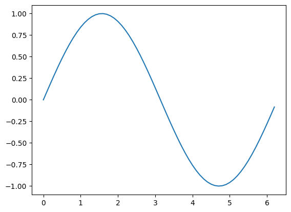
Later on in the course we’ll learn how to use matplotlib (a library for generating graphics and figures) and numpy a library for efficiently working with matrices and arrays. For now don’t worry about understanding the code above in detail. You can still play around with the contents of each line and see how it changes the figure. For example:

1. Change the 0 in np.arange(0, 2*np.math.pi, 0.1) to another number. What part of the graph does this affect?

2. Change the 2*np.math.pi in np.arange(0, 2*np.math.pi, 0.1) to another number. What part of the graph does this affect?

3. Change the 0.1 in np.arange(0, 2*np.math.pi, 0.1) to another number. What part of the graph does this affect?

4. Change the np.sin(x) to np.cos(x) in the line plt.plot(x, np.sin(x)). What other functions are supported?

5. What do you think the np.arange function does?

6. What do you think the plt.plot function does?

7. Which aspects of the code don’t you think you understand? Practice articulating your questions by separating out what you think you understand from what you think you don’t understand. Turn your confusion into askable questions!

If you’ve used a graphing calculator before, you might recognize some similarities between how you interacted with the graphing calculator to plot functions and the code you see above.

Notebooks of the Future

Not just for code:

• Markdown, HTML, LaTeX integration

• Slide shows

• Keep your notes alongside your analysis routines

• Embed images, videos, anything (it’s all just HTML + javascript)

Markdown

See this comprehensive guide to Markdown or tutorial. Here are some examples:

Emphasis

Here is one way to add emphasis to Markdown cell text.

Input	Output
Emphasis, aka italics, with *asterisks*.	Emphasis, aka italics, with asterisks.

Here is another way to add emphasis to Markdown cell text.

Input	Output
Strong emphasis, aka bold, with **asterisks**.	Strong emphasis, aka bold, with asterisks.

Here is another way to add emphasis to Markdown cell text.

Input	Output
Combined emphasis with ***asterisks***.	Combined emphasis with asterisks.

Here is one way to add strikethrough to Markdown cell text.

Input	Output
Strikethrough uses two tildes. ~~Scratch this.~~	Strikethrough uses two tildes. ~~Scratch this.~~

Links

Here is one way to insert hyperlinks into Markdown cells.

Input	Output
[I'm an inline-style link](https://www.google.com)	I’m an inline-style link

URLs and URLs in angle brackets will automatically get turned into links. http://www.example.com or http://www.example.com and sometimes example.com (but not on Github, for example).

Tables

Colons can be used to align columns (note that this may not render properly in the Jupyter Book website).

| Tables        | Are           | Cool  |
| :------------ |:-------------:| -----:|
| col 1 is      | left-aligned  |     A |
| col 3 is      | right-aligned |     B |
| col 2 is      | centered      |     C |

Tables	Are	Cool
col 1 is	left-aligned	A
col 3 is	right-aligned	B
col 2 is	centered	C

The outer pipes (|) are optional, and you don’t need to make the raw Markdown pretty. You can also use inline Markdown.

Markdown | Less | Pretty
--- | --- | ---
*Still* | `renders` | **nicely**
1 | 2 | 3

Markdown	Less	Pretty
Still	renders	nicely
1	2	3

Inserting images from web

Here is an example of inserting an image into a Markdown cell.

Input	Output


HTML Integration:

Here’s an example using HTML!

Input	Output
<font color=red>This is a</font> *markdown* **cell**!	This is a markdown cell!

LaTeX Integration:

Here’s an example using LaTeX

Input	Output
$\sum_{n=1}^{5}n$	\(\sum_{n=1}^{5}n\)

Multilingual!

Jupyter Notebooks support over 150+ languages!

These include:

• Julia

• Python

• R

• Javascript

Save notebooks in other formats and put them online

• Github automatically renders Jupyter Notebooks

• Online notebook viewer

• Output to PDF, HTML (including JavaScript)

• JupyterHub

Customize your notebook experience with extensions

• Table of Contents

• Execution time/Profiling

• Scratch Space

• Code/Section folding

• Look and feel (CSS+Javascript)

• Other notebook extensions

Additional Resources

• Eshin Jolly - Intro to Jupyter Notebooks

• Jake Vanderplas - Data Science Handbook

• Tal Yarkoni - Intro to Data Science w/ Python

• Yaroslav Halchenko - Intro to Programming for Psych/Neuro

• Awesome notebooks

• Neuroimaging in Python

• Google Colaboratory