Hypothesis Testing¶

This tutorial was inspired by and adapted from Shawn A. Rhoads’ PSYC 347 Course [CC BY-SA 4.0 License] and Russell Poldrack’s Statistical Thinking for the 21st Century [CC BY-NC 4.0].

Learning objectives¶

This notebook is intended to teach you basic python syntax for:

Independent samples t-tests
Paired samples t-tests

Independent samples t-tests¶

Now that we have basics of Python syntax, data processing, and data visualization down, we can move on to hypothesis testing. Hypothesis testing is a way to test whether a certain effect is present in a population. For example, we might want to test whether a certain drug is effective in treating a psychiatric condition. We can do this by comparing the mean of a certain measure (e.g., symptom severity) in a group of people who took the drug to the mean of the same measure in a group of people who did not take the drug (a good design would also used a randomized control trial for group selection). If the mean of the measure is significantly lower in the group that took the drug, we can conclude that the drug is effective in treating the condition.

We will apply this framework to compare means of two groups using independent samples t-tests.

# import our packages
import pandas as pd, numpy as np, matplotlib.pyplot as plt, seaborn as sns
from scipy.stats import ttest_ind, shapiro, levene, ttest_rel
from scipy import stats

Recall our data from the visualizations module. We explored the relationship between Depression and Loneliness. We found that there was a positive correlation between the two variables: As Depression increased, Loneliness also increased. However, we did not test whether this relationship was statistically significant. An independent samples t-test will allow us to test whether the mean differences in Loneliness between the High and Low Depression groups are statistically significant.

We will use the stats.ttest_ind() function from the scipy package to perform the t-test. This function takes two arrays as input and returns the t-statistic and p-value. The t-statistic is a measure of the difference between the two groups relative to the variance within each group. The p-value is the probability of observing a difference between the two groups as large as the one we observed if the null hypothesis is true. The null hypothesis is that there is no difference between the two groups. If the p-value is less than 0.05, we can reject the null hypothesis and conclude that there is a significant difference between the two groups.

our_data = pd.read_csv('https://raw.githubusercontent.com/Center-for-Computational-Psychiatry/course_spice/main/modules/resources/data/Banker_et_al_2022_QuestionnaireData_clean.csv')

# define groups
our_data['DepressionGroups'] = pd.cut(our_data['Depression'], 2, labels=['Low', 'High'])
group1 = our_data[our_data['DepressionGroups']=='High']
group2 = our_data[our_data['DepressionGroups']=='Low']

# t-test
t, p = ttest_ind(group1['Loneliness'], group2['Loneliness'])

if p < .05:
    print(f'T({(len(group1) + len(group2)) - 2})={t:.2f}, p={p}')

T(1088)=17.21, p=7.0949774878784104e-59

We can see that the p-value is less than 0.05, so we can reject the null hypothesis and conclude that there is a significant difference between the two groups. We can also see that the t-statistic is positive, which means that the mean Loneliness score is higher in the High Depression group than in the Low Depression group. This is consistent with our visualization from the previous module.

Easy, right? But what does this all mean?

The p-value is the probability of observing a difference between the two groups as large as the one we observed if the null hypothesis is true. The null hypothesis is that there is no difference between the two groups. If the p-value is less than 0.001, we can reject the null hypothesis and conclude that there is a significant difference between the two groups with 99.9% confidence. (If the p-value is less than 0.01, we can reject the null hypothesis and conclude that there is a significant difference between the two groups with 99% confidence. If the p-value is less than 0.05, we can reject the null hypothesis and conclude that there is a significant difference between the two groups with 95% confidence.)

…okay, great! But we can do better right?

Let’s do an even deeper dive¶

The independent samples t-test is a statistical test used to determine whether there is a significant difference between the means of two independent groups. It is commonly used in research to compare the means of two groups and determine whether the difference is statistically significant.

The t-test is based on the t-distribution, which is a probability distribution that is similar to the normal distribution but is better suited for small sample sizes. The t-distribution has a mean of 0 and a standard deviation of 1, and its shape depends on the degrees of freedom.

The formula for the independent samples t-test is:

\[t = \frac{\bar{x}_1 - \bar{x}_2}{\sqrt{\frac{s_1^2}{n_1} + \frac{s_2^2}{n_2}}}\]

Where:

\(\bar{x}_1\) and \(\bar{x}_2\) are the sample means for the two groups
\(s_1\) and \(s_2\) are the sample standard deviations for the two groups
\(n_1\) and \(n_2\) are the sample sizes for the two groups
\(t\) is the t-statistic

Assumptions for an Independent Samples t-Test¶

In order to run an independent samples t-test, we must check that the following conditions are met:

Independence: The two samples are independent of each other. This means that the observations in one sample are not related to the observations in the other sample.
Normality: The populations from which the samples are drawn are normally distributed. This assumption is important because the t-test is sensitive to departures from normality, especially for small sample sizes.
Equal variances: The two populations have equal variances. This assumption is important because the t-test assumes that the variances of the two populations are equal. If the variances are unequal, the t-test may not be appropriate and an alternative test, such as the Welch’s t-test, may be used instead.

If these assumptions are not met, the results of the t-test may not be valid. In practice, it is important to check these assumptions before conducting a t-test. There are several methods for checking normality and equal variances, such as visual inspection of histograms and boxplots, as well as statistical tests such as the Shapiro-Wilk test and the Levene’s test.

We can use the stats.shapiro() function from the scipy package to test for normality. This function takes an array as input and returns the test statistic and p-value. The test statistic is a measure of the difference between the observed data and the expected data under the null hypothesis. The p-value is the probability of observing a test statistic as extreme as the one we observed if the null hypothesis is true. If the p-value is less than 0.05, we can reject the null hypothesis and conclude that the data are not normally distributed.

We can use the stats.levene() function from the scipy package to test for equal variances. This function takes two arrays as input and returns the test statistic and p-value. The test statistic is a measure of the difference between the observed data and the expected data under the null hypothesis. The p-value is the probability of observing a test statistic as extreme as the one we observed if the null hypothesis is true. If the p-value is less than 0.05, we can reject the null hypothesis and conclude that the variances are not equal.

# Check for normality
normality1 = shapiro(group1['Loneliness']).pvalue > 0.05
normality2 = shapiro(group2['Loneliness']).pvalue > 0.05

# Check for equal variances
equal_variances = levene(group1['Loneliness'], group2['Loneliness']).pvalue > 0.05

# Print the results
print(f"Normality: {normality1}, {normality2}")
print(f"Equal variances: {equal_variances}")

Normality: False, False
Equal variances: False

We see that both of our artifical groups have equal variances but only one of them is normally distributed. For the sake of this tutorial, we will continue with the t-test but we should be aware that the results may not be valid.

Calculating the Mean and Variance for Each Group¶

Before we can calculate the t-statistic, we need to calculate the mean and variance for each group. In our case, we have two groups: the depression group and the non-depression group. We will use the numpy library to calculate the mean and variance for each group.

# Extract the 'Loneliness' values for the high and low depression groups using boolean indexing
high_depression_group = our_data[our_data['DepressionGroups'] == 'High']['Loneliness']
low_depression_group = our_data[our_data['DepressionGroups'] == 'Low']['Loneliness']

# Calculate the mean for each group using numpy's mean function
high_depression_mean = np.mean(high_depression_group)
low_depression_mean = np.mean(low_depression_group)

# Calculate the variance for each group using numpy's var function
# Set the ddof parameter to 1 to calculate the unbiased estimate of the variance
high_depression_var = np.var(high_depression_group, ddof=1)
low_depression_var = np.var(low_depression_group, ddof=1)

print(f"High depression group mean: {high_depression_mean:.2f}")
print(f"High depression group variance: {high_depression_var:.2f}")

print(f"Low depression group mean: {low_depression_mean:.2f}")
print(f"Low depression group variance: {low_depression_var:.2f}")

High depression group mean: 22.50
High depression group variance: 13.53
Low depression group mean: 17.96
Low depression group variance: 16.29

Here, we first extract the Loneliness values for each group using boolean indexing. We then use the numpy functions mean() and var() to calculate the mean and variance for each group. Note that we set the ddof parameter to 1 to calculate the unbiased estimate of the variance.

In the next section, we will use these values to calculate the pooled variance.

Calculating the Pooled Variance¶

The next step in the independent samples t-test is to calculate the pooled variance. The pooled variance is a weighted average of the variances of the two groups, and it is used to estimate the variance of the population from which the samples were drawn.

The formula for the pooled variance is:

\[s_p^2 = \frac{(n_1 - 1)s_1^2 + (n_2 - 1)s_2^2}{n_1 + n_2 - 2}\]

Where:

\(s_1^2\) and \(s_2^2\) are the sample variances for the two groups
\(n_1\) and \(n_2\) are the sample sizes for the two groups
\(s_p^2\) is the pooled variance

We can calculate the pooled variance using the following code:

# Get the group sizes using the len function
n1 = len(high_depression_group)
n2 = len(low_depression_group)
 
# Calculate the pooled variance using the formula
pooled_var = ((n1 - 1) * high_depression_var + (n2 - 1) * low_depression_var) / (n1 + n2 - 2)

print(f"Pooled variance: {pooled_var:.2f}")

Pooled variance: 15.50

Calculating the t-Statistic¶

Now that we have calculated the mean and variance for each group, as well as the pooled variance, we can calculate the t-statistic using the formula we introduced earlier:

\[t = \frac{\bar{x}_1 - \bar{x}_2}{\sqrt{\frac{s_p^2}{n_1} + \frac{s_p^2}{n_2}}}\]

Where:

\(\bar{x}_1\) and \(\bar{x}_2\) are the sample means for the two groups
\(s_p^2\) is the pooled variance
\(n_1\) and \(n_2\) are the sample sizes for the two groups
\(t\) is the t-statistic

We can calculate the t-statistic using the following code:

# Calculate the t-statistic using the formula
t_statistic = (high_depression_mean - low_depression_mean) / np.sqrt(pooled_var * (1/n1 + 1/n2))

print(f"t-statistic: {t_statistic:.2f}")

t-statistic: 17.21

Here, we use the formula to calculate the t-statistic, where high_depression_mean and low_depression_mean are the sample means for the two groups that we calculated earlier, and pooled_var is the pooled variance that we calculated in the previous section.

Pretty cool how it matches the scipy output from earlier, right?

In the next section, we will calculate the degrees of freedom and the critical value for t, which we will use to determine whether the difference between the two groups is statistically significant.

Calculating Degrees of Freedom and Critical Value¶

The degrees of freedom (df) is a number that tells us how much information we have in our data. It’s like the number of “free” values that we can choose when we calculate a statistic. In the case of the t-test, the degrees of freedom is equal to the sum of the sample sizes minus 2.

df = n1 + n2 - 2
print(f"Degrees of freedom: {df}")

Degrees of freedom: 1088

We use the degrees of freedom to calculate the critical value for t, which helps us decide if the difference between two groups is important or not. The higher the degrees of freedom, the more reliable our results are.

The critical value is a number that helps us decide if the difference between two groups is important or not. It’s like a line that separates the “important” differences from the “not important” differences. We use this line to make a decision about whether the difference we see is real or just due to chance. It is also determined by the significance level, denoted by alpha (α), which is the probability of rejecting the null hypothesis when it is actually true. The most commonly used significance level is 0.05, which means that there is a 5% chance of rejecting the null hypothesis when it is actually true.

If the absolute value of the t-statistic is greater than the critical value, then we reject the null hypothesis and conclude that the difference between the two groups is statistically significant. If the absolute value of the t-statistic is less than the critical value, then we fail to reject the null hypothesis and conclude that the difference between the two groups is not statistically significant.

We can use the degrees of freedom to look up the critical value for t in a t-distribution table. Alternatively, we can use the t.ppf() function from the scipy.stats module to calculate the critical value directly. The t.ppf() function takes two arguments: the significance level (alpha) and the degrees of freedom (df).

A t-distribution is a probability distribution that is used in hypothesis testing when the sample size is small or the population standard deviation is unknown. It is similar to a normal distribution, but with heavier tails and a flatter peak.

The shape of the t-distribution depends on the degrees of freedom, which is the number of independent observations in the sample. As the degrees of freedom increase, the t-distribution approaches a normal distribution.

# Calculate the critical value for t
alpha = 0.05  # significance level
t_critical = stats.t.ppf(alpha, df)

# compute the confidence intervals too
t_conf_int = t_critical * np.sqrt(pooled_var * (1/n1 + 1/n2))

print(f"Critical value for t: {t_critical:.2f}")

Critical value for t: -1.65

Here, we use the t.ppf() function to calculate the critical value for t at a significance level of 0.05. The df variable is the degrees of freedom that we calculated earlier.

In the next section, we will compare the t-statistic to the critical value to determine whether the difference between the two groups is statistically significant.

The t.ppf(alpha, df) function returns the critical value for a t-distribution with df degrees of freedom at a given significance level alpha.

To visualize how this function works, we can plot a t-distribution with df degrees of freedom and shade the rejection region based on the significance level alpha. The critical value is the boundary between the rejection region and the non-rejection region.

Here’s an example code snippet that generates a plot of a t-distribution with our degrees of freedom and a significance level of 0.05:

# Set the degrees of freedom and significance level
df = n1 + n2 - 2
alpha = 0.05

# Generate x values for the t-distribution
x = np.linspace(-20, 20, 1000)

# Calculate the t-distribution for the given degrees of freedom
t_dist = stats.t(df)

# Calculate the critical value for the given significance level and degrees of freedom
t_critical = t_dist.ppf(1 - alpha/2)

# Shade the rejection region and add a vertical line at the critical t-value
if t_critical > 0:
    plt.fill_between(x, t_dist.pdf(x), where=(x > t_critical), color='red', alpha=0.2)
    plt.axvline(x=t_critical, color='red', linestyle='--', label='critical t')
else:
    plt.fill_between(x, t_dist.pdf(x), where=(x < -t_critical), color='red', alpha=0.2)
    plt.axvline(x=-t_critical, color='red', linestyle='--', label='critical t')

# Plot the t-distribution
plt.plot(x, t_dist.pdf(x))

# Plot the t-statistic for comparison
plt.axvline(x=t_statistic, color='black', linestyle='-', label='t-statistic')

# Add labels and title
plt.xlabel('t')
plt.ylabel('Probability density')
plt.title(f't distribution with {df} degrees of freedom')

plt.legend();

# Show the plot
plt.show()

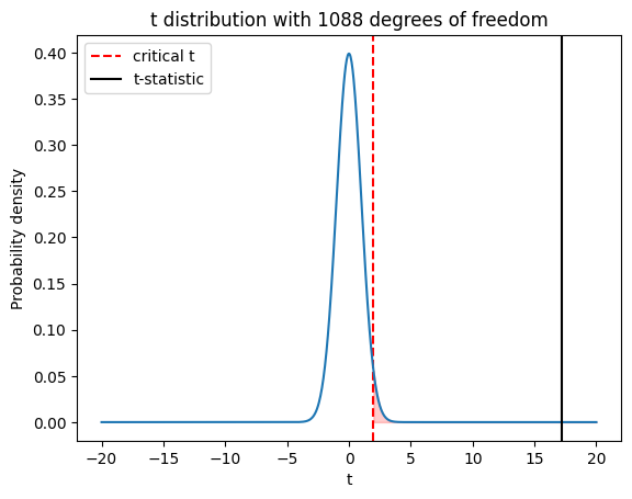
Play around with this code! What happens if you change the alpha value? What happens if you change the degrees of freedom (df)?

# Insert your code here

Comparing the t-Statistic with the Critical Value¶

Now that we have calculated the critical value, we can compare it with the t-statistic. If the absolute value of the t-statistic is greater than the critical value, then we reject the null hypothesis and conclude that the means of the two groups are statistically different. If the absolute value of the t-statistic is less than or equal to the critical value, then we fail to reject the null hypothesis and conclude that there is not enough evidence to support a difference between the means.

In the code snippet earlier, we calculated the critical value for t using the ppf() function. We also visualized this. We can now compare this critical value with the actual t-statistic to determine whether the difference between the means of the two groups is statistically significant.

# Calculate the critical value for t
t_critical = stats.t.ppf(1 - alpha/2, df)

# Calculate the t-statistic
t_statistic = (high_depression_mean - low_depression_mean) / np.sqrt(pooled_var * (1/n1 + 1/n2))

# Compare the t-statistic with the critical value
if abs(t_statistic) > t_critical:
    print("The difference between the means of the two groups is statistically significant at alpha=0.05")
else:
    print("There is not enough evidence to support a difference between the means of the two groups at alpha=0.05.")

The difference between the means of the two groups is statistically significant at alpha=0.05

Computing the standard error and confidence intervals¶

Using the critical t-value and specified alpha level, we can also compute the standard error and confidence intervals for the difference between the means of the two groups.

The standard error is the standard deviation of the sampling distribution of the difference between the means of the two groups. It is calculated using the following formula:

\[SE = \sqrt{\frac{s_1^2}{n_1} + \frac{s_2^2}{n_2}}\]

Where:

\(s_1^2\) and \(s_2^2\) are the sample variances for the two groups
\(n_1\) and \(n_2\) are the sample sizes for the two groups

The confidence interval is a range of values that we can be confident contains the true difference between the means of the two groups. It is calculated using the following formula:

\[CI = (\bar{x}_1 - \bar{x}_2) \pm t_{\alpha/2, df} \times SE\]

Where:

\(\bar{x}_1\) and \(\bar{x}_2\) are the sample means for the two groups
\(t_{\alpha/2, df}\) is the critical value for t at a given significance level and degrees of freedom

Here, we use the formulas to calculate the standard error and confidence intervals for the difference between the means of the two groups.

# calculate the standard error of the mean difference
standard_error = np.sqrt(pooled_var * (1/n1 + 1/n2))

# calculate the margin of error
margin_of_error = t_critical * standard_error

# calculate the confidence interval
lower_bound = t_statistic - margin_of_error
upper_bound = t_statistic + margin_of_error

print(f"Confidence interval: [{lower_bound:.2f}, {upper_bound:.2f}]")

Confidence interval: [16.69, 17.72]

Computing the P-Value¶

We can also compute the p-value to determine the statistical significance of the difference between the means of the two groups. The p-value is the probability of observing a t-statistic as extreme or more extreme than the one calculated, assuming that the null hypothesis is true.

To compute the p-value, we can use the sf() function from the scipy.stats.t module. The sf() function calculates the survival function, which is equal to 1 minus the cumulative distribution function (CDF). The CDF gives the probability of observing a t-statistic less than or equal to the one calculated, while the survival function gives the probability of observing a t-statistic greater than the one calculated.

To compute the p-value, we need to calculate the survival function for the absolute value of the t-statistic and multiply it by 2. This is because the t-distribution is symmetric around 0, so we need to account for the possibility of observing a t-statistic in either tail of the distribution.

p_value = 2 * stats.t.sf(abs(t_statistic), df)

# Print the p-value
print(f"p-value: {p_value}")

p-value: 7.0949774878784104e-59

The p-value is less than 0.05, so we reject the null hypothesis and conclude that the difference between the means of the two groups is statistically significant.

Isn’t it cool that we got the same result as the ttest_ind() function from the scipy.stats module?

Putting it all together¶

Now that we have calculated the t-statistic, the critical value, and the p-value, we can put it all together to make a decision about whether the difference between the means of the two groups is statistically significant.

# Extract the 'Loneliness' values for the high and low depression groups using boolean indexing
high_depression_group = our_data[our_data['DepressionGroups'] == 'High']['Loneliness']
low_depression_group = our_data[our_data['DepressionGroups'] == 'Low']['Loneliness']

# Calculate the mean for each group using numpy's mean function
high_depression_mean = np.mean(high_depression_group)
low_depression_mean = np.mean(low_depression_group)

# Calculate the variance for each group using numpy's var function
# Set the ddof parameter to 1 to calculate the unbiased estimate of the variance
high_depression_var = np.var(high_depression_group, ddof=1)
low_depression_var = np.var(low_depression_group, ddof=1)

# Get the group sizes using the len function
n1 = len(high_depression_group)
n2 = len(low_depression_group)

# Calculate the pooled variance using the formula
pooled_var = ((n1 - 1) * high_depression_var + (n2 - 1) * low_depression_var) / (n1 + n2 - 2)

# Calculate the t-statistic using the formula
t_statistic = (high_depression_mean - low_depression_mean) / np.sqrt(pooled_var * (1/n1 + 1/n2))

# Calculate the degrees of freedom
df = n1 + n2 - 2

# calculate the critical value for t
t_critical = stats.t.ppf(1 - alpha/2, df)

# calculate the standard error of the mean difference
standard_error = np.sqrt(pooled_var * (1/n1 + 1/n2))

# calculate the margin of error
margin_of_error = t_critical * standard_error

# calculate the confidence interval
lower_bound = t_statistic - margin_of_error
upper_bound = t_statistic + margin_of_error

# Calculate the p-value
p_value = 2 * stats.t.sf(abs(t_statistic), df)

# Print the t-statistic and p-value
print(f"t-statistic: {t_statistic:.2f}, 95% CI: [{lower_bound:.2f}, {upper_bound:.2f}], p-value: {p_value}")

t-statistic: 17.21, 95% CI: [16.69, 17.72], p-value: 7.0949774878784104e-59

Now that we understand all of the code behind the ttest_ind() function, there is no need to use all of this code in our own projects. We can benefit (and save time) by just using the ttest_ind() function from the scipy.stats module (like from earlier)

# ttest_ind function
t_statistic, p_value = ttest_ind(high_depression_group, low_depression_group)
print(f"t-statistic: {t_statistic:.2f}, p-value: {p_value}")

t-statistic: 17.21, p-value: 7.0949774878784104e-59

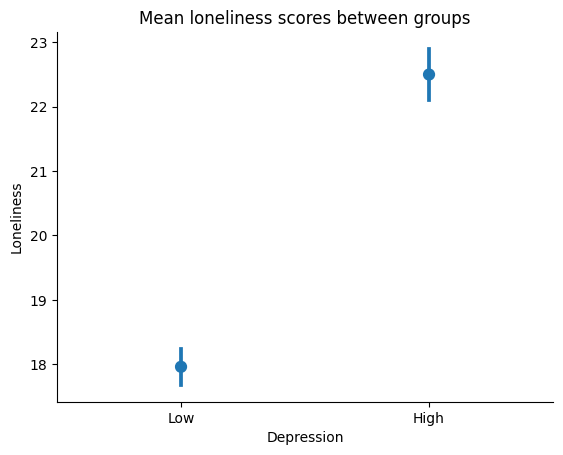
Visualizing our results¶

We can plot the means of our two groups on a point plot to visualize the difference between them.

# plot means, do not join because they are independent samples
ax = sns.pointplot(x='DepressionGroups', y='Loneliness', data=our_data, join=False) 

# we can also add a title and labels to the axes
ax.set_title('Mean loneliness scores between groups')
ax.set_xlabel('Depression')
ax.set_ylabel('Loneliness')

# we can also tidy up some more by removing the top and right spines
sns.despine()

# we will use the `show()` function to plot within the notebook
plt.show()

Paired samples t-tests¶

In the previous section, we learned how to perform an independent-samples t-test in Python. In this section, we will learn how to perform a paired samples t-test in Python. A paired samples t-test is used when we want to compare the means of two groups that are related to each other.

\[t = \frac{\bar{d}}{s_d/\sqrt{n}}\]

where \(\bar{d}\) is the mean difference between the paired observations, \(s_d\) is the standard deviation of the differences, and \(n\) is the number of pairs.

The paired samples t-test compares the mean difference between the paired observations to zero, under the null hypothesis that there is no significant difference between the two samples. If the absolute value of the calculated t-statistic is greater than the critical t-value for the desired significance level and degrees of freedom, we reject the null hypothesis and conclude that there is a significant difference between the two samples.

This is different from an independent samples t-test (from earlier), which is used to compare the means of two separate groups of data. For example, let’s say we want to compare depression scores of patients from two different hospitals. If we use an independent samples t-test, we would take a sample of patients from each hospital and compare the means of the two samples. This test would NOT be applicable if we wanted to compare the means depression scores for patients who received a treatment. In this case, we would need to use a paired samples t-test to measure the difference in depression scores for each patient before and after receiving the treatment.

In other words, the independent samples t-test assumes that the two groups of data are independent and unrelated, while the paired samples t-test assumes that the two groups of data are related or paired in some way.

The paired samples t-test is often used when we want to compare the same group of individuals or objects at two different points in time, or when we want to compare two different treatments applied to the same group of individuals or objects.

Both tests are used to determine whether there is a significant difference between the means of two groups of data, but they are used in different situations depending on the nature of the data.

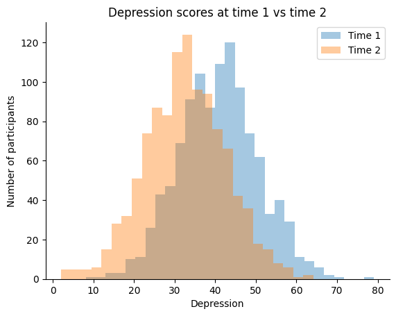
Let’s work through the second example by simulating a fake Depression scores for each participant. Let’s assume that the new depression scores were measured after participants received a treatment.

# Create fake time 1 and 2 depression score with different means
np.random.seed(42)
time1_depression = np.random.normal(loc=40.54, scale=10, size=len(our_data))
time2_depression = np.random.normal(loc=32.25, scale=10, size=len(our_data))

# Let's plot our means to see how they look
ax = sns.distplot(time1_depression, kde=False, label='Time 1')
ax = sns.distplot(time2_depression, kde=False, label='Time 2')

# we can also add a title and labels to the axes
ax.set_title('Depression scores at time 1 vs time 2')
ax.set_xlabel('Depression')
ax.set_ylabel('Number of participants')

plt.legend()

# we can also tidy up some more by removing the top and right spines
sns.despine()

# we will use the `show()` function to plot within the notebook
plt.show()

We can run a paired samples t-test in Python using the ttest_rel() function from the scipy.stats module. The ttest_rel() function takes two arrays of observations as arguments and returns the t-statistic and p-value.

# paired samples t-test
t, p = ttest_rel(time1_depression, time2_depression)

if p < .05:
    print(f'T({len(time1_depression) - 1}) = {t:.2f}, p = {p}')

T(1089) = 19.19, p = 5.922994536108181e-71

Assumptions for a Paired Samples t-Test¶

The assumptions for a paired samples t-test is similar to the assumptions for an independent samples t-test. The major difference is that the paired samples t-test assumes that the two samples are related or paired in some way.

Calculating the Mean and Variance¶

Note that we only have one sample, so we only need to compute the difference between the two time points.

Let’s start by calculating the mean and variance for each time point. We can do this using the mean() and var() functions from the numpy module.

# calculate the difference between the two time points
time_diff = time1_depression - time2_depression
mean_diff = np.mean(time_diff)

# calculate the standard deviation of the difference
time_diff_std = np.std(time_diff, ddof=1)   

# print the mean and variance of the difference 
print(f"Mean Difference: {mean_diff:.2f}, Standard Deviation: {time_diff_std:.2f}")

Mean Difference: 8.20, Standard Deviation: 14.10

Calculate the t-Statistic¶

Now that we have calculated the mean and variance for each time point, we can calculate the t-statistic. We can do this using the formula from above.

# calculate the sample size
n = len(time1_depression)

# calculate the t-statistic
t_stat = mean_diff / (time_diff_std / np.sqrt(n))

print(f"t-statistic: {t_stat:.2f}")

t-statistic: 19.19

Calculating Degrees of Freedom and Critical Value¶

Now that we have calculated the t-statistic, we can calculate the degrees of freedom and the critical value. We can do this using the t.ppf() function from the scipy.stats.t module. The t.ppf() function takes two arguments: the significance level and the degrees of freedom. The t.ppf() function returns the critical value for the given significance level and degrees of freedom.

# calculate the degrees of freedom
df = n - 1

# calculate the critical value
t_critical = stats.t.ppf(1 - alpha/2, df)

print(f"Critical value: {t_critical:.2f}")

Critical value: 1.96

Computing the standard error and confidence intervals¶

# calculate the standard error of the mean difference
standard_error = time_diff_std / np.sqrt(n)

# calculate the margin of error
margin_of_error = t_critical * standard_error

# calculate the confidence interval
lower_bound = t_stat - margin_of_error
upper_bound = t_stat + margin_of_error

print(f"Confidence interval: [{lower_bound:.2f}, {upper_bound:.2f}]")

Confidence interval: [18.36, 20.03]

Comparing the t-Statistic with the Critical Value¶

After calculating the t-statistic for the paired samples t-test, we can compare it with the critical value from the t-distribution to determine whether the difference between the paired samples is statistically significant.

The critical value is determined by the significance level (alpha) and the degrees of freedom (df), which is equal to the sample size minus one.

If the absolute value of the t-value is greater than the critical value, we can reject the null hypothesis and conclude that the difference between the paired samples is statistically significant at the given significance level. Otherwise, we fail to reject the null hypothesis and conclude that there is not enough evidence to support a significant difference between the paired samples.

# compare the t-value with the critical value
if abs(t_stat) > t_critical:
    print("The difference between the means of the two time points is statistically significant at alpha=0.05")
else:
    print("There is not enough evidence to support a difference between the means of the two time points at alpha=0.05.")

The difference between the means of the two time points is statistically significant at alpha=0.05

Computing the P-Value¶

Finally, we can compute the p-value to determine the statistical significance of the difference between the paired samples. The p-value is the probability of observing a t-statistic as extreme or more extreme than the one calculated, assuming that the null hypothesis is true.

# compute the p-value
p_value = 2 * stats.t.sf(abs(t_stat), df)

# print the p-value
print(f"p-value: {p_value}")

p-value: 5.922994536108181e-71

Putting it all together¶

Now that we have calculated the t-statistic, the critical value, and the p-value, we can put it all together to make a decision about whether the difference between the means of the two groups is statistically significant.

# Create fake time 1 and 2 depression score with different means
np.random.seed(42)
time1_depression = np.random.normal(loc=40.54, scale=10, size=len(our_data))
time2_depression = np.random.normal(loc=32.25, scale=10, size=len(our_data))

# calculate the difference between the two time points
time_diff = time1_depression - time2_depression
mean_diff = np.mean(time_diff)

# calculate the standard deviation of the difference
time_diff_std = np.std(time_diff, ddof=1)   

# calculate the sample size
n = len(time1_depression)

# calculate the t-statistic
t_stat = mean_diff / (time_diff_std / np.sqrt(n))

# calculate the degrees of freedom
df = n - 1

# calculate the critical value
t_critical = stats.t.ppf(1 - alpha/2, df)

# calculate the standard error of the mean difference
standard_error = time_diff_std / np.sqrt(n)

# calculate the margin of error
margin_of_error = t_critical * standard_error

# calculate the confidence interval
lower_bound = t_stat - margin_of_error
upper_bound = t_stat + margin_of_error

# calculate the critical value
p_value = 2 * stats.t.sf(abs(t_stat), df)

# Print the t-statistic and p-value
print(f"t-statistic: {t_stat:.2f}, 95% CI: [{lower_bound:.2f}, {upper_bound:.2f}], p-value: {p_value}")

t-statistic: 19.19, 95% CI: [18.36, 20.03], p-value: 5.922994536108181e-71

Now that we understand all of the code behind the ttest_rel() function, there is no need to use all of this code in our own projects. We can benefit (and save time) by just using the ttest_rel() function from the scipy.stats module (like from earlier)

# ttest_ind function
t_statistic, p_value = ttest_rel(time1_depression, time2_depression)

print(f"t-statistic: {t_statistic:.2f}, p-value: {p_value}")

t-statistic: 19.19, p-value: 5.922994536108181e-71

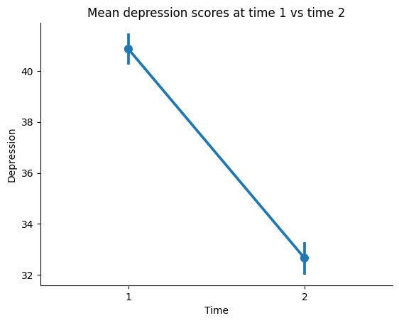
Visualizing our results¶

Let’s plot a pointplot to visualize the difference between the two time points. We can do this using the pointplot() function from the seaborn module.

# let's create a new datafame in long form with the time points as a column
our_data_long = pd.DataFrame({'Depression': np.concatenate([time1_depression, time2_depression]), 'Time': ['1'] * len(time1_depression) + ['2'] * len(time2_depression)})
ax = sns.pointplot(x='Time', y='Depression', data=our_data_long)

# we can also add a title and labels to the axes
ax.set_title('Mean depression scores at time 1 vs time 2')
ax.set_xlabel('Time')
ax.set_ylabel('Depression')

# we can also tidy up some more by removing the top and right spines
sns.despine()

# we will use the `show()` function to plot within the notebook
plt.show()

Next steps¶

In this tutorial, we learned how to perform a two-sample t-test in Python from scratch. We also learned how to use the ttest_ind() function from the scipy.stats module to perform a two-sample t-test.

We also learned how to perform a paired samples t-test in Python from scratch. We also learned how to use the ttest_rel() function from the scipy.stats module to perform a paired samples t-test.

You can read more about null hypothesis testing and t-tests in the following resources:

Now, try this for yourself with different variables. Create new independent groups and explore whether there are differences between them.

# Insert your code here

Hypothesis Testing

Contents

Hypothesis Testing¶

Learning objectives¶

Independent samples t-tests¶

Let’s do an even deeper dive¶

Assumptions for an Independent Samples t-Test¶

Calculating the Mean and Variance for Each Group¶

Calculating the Pooled Variance¶

Calculating the t-Statistic¶

Calculating Degrees of Freedom and Critical Value¶

Comparing the t-Statistic with the Critical Value¶

Computing the standard error and confidence intervals¶

Computing the P-Value¶

Putting it all together¶

Visualizing our results¶

Paired samples t-tests¶

Assumptions for a Paired Samples t-Test¶

Calculating the Mean and Variance¶

Calculate the t-Statistic¶

Calculating Degrees of Freedom and Critical Value¶

Computing the standard error and confidence intervals¶

Comparing the t-Statistic with the Critical Value¶

Computing the P-Value¶

Putting it all together¶

Visualizing our results¶

Next steps¶