Numerical Operations

This tutorial was inspired by and adapted from Shawn A. Rhoads’ PSYC 347 Course [CC BY-SA 4.0 License] and NumPy Basics [NumPy license].

Learning objectives

This notebook is intended to teach you basic python syntax for:

1. Basic mathematical operations

2. Working with arrays

One important package for numerical operations in python is numpy. NumPy is a package that provides a multidimensional array object, various derived objects (such as masked arrays and matrices), and an assortment of routines for fast operations on arrays, including mathematical, logical, shape manipulation, sorting, selecting, basic linear algebra, basic statistical operations, random simulations, and much more.

# Before we start, let's import numpy as np
import numpy as np

What’s the difference between a Python list and a NumPy array?

NumPy gives you an enormous range of fast and efficient ways of creating arrays and manipulating numerical data inside them. While a Python list can contain different data types within a single list, all of the elements in a NumPy array should be homogeneous. The mathematical operations that are meant to be performed on arrays would be extremely inefficient if the arrays weren’t homogeneous.

Why use NumPy?

NumPy arrays are faster and more compact than Python lists. An array consumes less memory and is convenient to use. NumPy uses much less memory to store data and it provides a mechanism of specifying the data types. This allows the code to be optimized even further. What is an array?

An array is a central data structure of the NumPy library. An array is a grid of values and it contains information about the raw data, how to locate an element, and how to interpret an element. It has a grid of elements that can be indexed in various ways. The elements are all of the same type, referred to as the array dtype.

An array can be indexed by a tuple of nonnegative integers, by booleans, by another array, or by integers. The rank of the array is the number of dimensions. The shape of the array is a tuple of integers giving the size of the array along each dimension.

One way we can initialize NumPy arrays is from Python lists, using nested lists for two- or higher-dimensional data.

For example:

a1 = np.array([1, 2, 3, 4, 5, 6])

or

a2 = np.array([[1, 2, 3, 4], [5, 6, 7, 8], [9, 10, 11, 12]])

We can access the elements in the array using square brackets. When you’re accessing elements, remember that indexing in NumPy starts at 0. That means that if you want to access the first element in your array, you’ll be accessing element “0”.

print(a2[0])

[1 2 3 4]

More information about arrays

You might occasionally hear an array referred to as a “ndarray,” which is shorthand for “N-dimensional array.” An N-dimensional array is simply an array with any number of dimensions. You might also hear 1-D, or one-dimensional array, 2-D, or two-dimensional array, and so on. The NumPy ndarray class is used to represent both matrices and vectors. A vector is an array with a single dimension (there’s no difference between row and column vectors), while a matrix refers to an array with two dimensions. For 3-D or higher dimensional arrays, the term tensor is also commonly used.

What are the attributes of an array?

An array is usually a fixed-size container of items of the same type and size. The number of dimensions and items in an array is defined by its shape. The shape of an array is a tuple of non-negative integers that specify the sizes of each dimension.

In NumPy, dimensions are called axes. This means that if you have a 2D array that looks like this::

[[0., 0., 0.], [1., 1., 1.]]

Your array has 2 axes. The first axis has a length of 2 and the second axis has a length of 3.

Just like in other Python container objects, the contents of an array can be accessed and modified by indexing or slicing the array. Unlike the typical container objects, different arrays can share the same data, so changes made on one array might be visible in another.

Array attributes reflect information intrinsic to the array itself. If you need to get, or even set, properties of an array without creating a new array, you can often access an array through its attributes.

How to create a basic array

All you need to do to create a simple array is pass a list to the function np.array() (like we do above). You can visualize your array this way:

Besides creating an array from a sequence of elements, you can easily create an array filled with 0’s:

np.zeros(2)

array([0., 0.])

Or an array filled with 1’s:

np.ones(8)

array([1., 1., 1., 1., 1., 1., 1., 1.])

Or even an empty array! The function empty creates an array whose initial content is random and depends on the state of the memory. The reason to use empty over zeros (or something similar) is speed - just make sure to fill every element afterwards!

# Create an empty array with 4 elements
np.empty(4)

array([4.64643346e-310, 0.00000000e+000, 1.58101007e-322, 0.00000000e+000])

You can create an array with a range of elements:

np.arange(6)

array([0, 1, 2, 3, 4, 5])

And even an array that contains a range of evenly spaced intervals. To do this, you will specify the first number, last number, and the step size.

np.arange(2, 9, 2)

array([2, 4, 6, 8])

You can also use np.linspace() to create an array with values that are spaced linearly in a specified interval

np.linspace(0, 10, num=5)

array([ 0. ,  2.5,  5. ,  7.5, 10. ])

Specifying your data type

While the default data type is floating point (np.float64), you can explicitly specify which data type you want using the dtype keyword.

x = np.ones(2, dtype=np.int64)
x

array([1, 1])

Adding, removing, and sorting elements

Sorting an element is simple with np.sort(). You can specify the axis, kind, and order when you call the function.

If you start with this array

arr = np.array([2, 1, 5, 3, 7, 4, 6, 8])

You can quickly sort the numbers in ascending order with

np.sort(arr)

array([1, 2, 3, 4, 5, 6, 7, 8])

If you start with these arrays:

a = np.array([1, 2, 3, 4])
b = np.array([5, 6, 7, 8])

You can concatenate them with np.concatenate()

c = np.concatenate((a, b))
c

array([1, 2, 3, 4, 5, 6, 7, 8])

Or, if you start with these arrays:

x = np.array([[1, 2], [3, 4]])
y = np.array([[5, 6]])

You can concatenate them with:

np.concatenate((x, y), axis=0)

array([[1, 2],
       [3, 4],
       [5, 6]])

In order to remove elements from an array, it’s simple to use indexing to select the elements that you want to keep. For example, we can select the first five elements of the array like this:

c[0:5]

array([1, 2, 3, 4, 5])

NumPy arrays also have the following attributes:

• ndarray.ndim will tell you the number of axes, or dimensions, of the array.

• ndarray.size will tell you the total number of elements of the array. This is the product of the elements of the array’s shape.

• ndarray.shape will display a tuple of integers that indicate the number of elements stored along each dimension of the array. If, for example, you have a 2-D array with 2 rows and 3 columns, the shape of your array is (2, 3).

For example:

array_example = np.array([[[0, 1, 2, 3],
                           [4, 5, 6, 7]],
                          [[0, 1, 2, 3],
                           [4, 5, 6, 7]],
                          [[0 ,1 ,2, 3],
                           [4, 5, 6, 7]]])

To find the number of dimensions of the array, run:

array_example.ndim

To find the total number of elements in the array, run:

array_example.size

24

And to find the shape of your array, run:

array_example.shape

(3, 2, 4)

Can you reshape an array?

Yes!

Using arr.reshape() will give a new shape to an array without changing the data. Just remember that when you use the reshape method, the array you want to produce needs to have the same number of elements as the original array. If you start with an array with 12 elements, you’ll need to make sure that your new array also has a total of 12 elements.

If you start with this array:

a = np.arange(6)
a

array([0, 1, 2, 3, 4, 5])

You can use reshape() to reshape your array. For example, you can reshape this array to an array with three rows and two columns:

b = a.reshape(3, 2)
print(b)

[[0 1]
 [2 3]
 [4 5]]

Converting a 1D array into a 2D array (how to add a new axis to an array)

You can use np.newaxis and np.expand_dims to increase the dimensions of your existing array.

Using np.newaxis will increase the dimensions of your array by one dimension when used once. This means that a 1D array will become a 2D array, a 2D array will become a 3D array, and so on.

For example, if you start with this array:

a = np.array([1, 2, 3, 4, 5, 6])
a.shape

(6,)

You can use np.newaxis to add a new axis:

a2 = a[np.newaxis, :]
a2.shape

(1, 6)

You can explicitly convert a 1D array with either a row vector or a column vector using np.newaxis. For example, you can convert a 1D array to a row vector by inserting an axis along the first dimension:

row_vector = a[np.newaxis, :]
row_vector.shape

(1, 6)

Or, for a column vector, you can insert an axis along the second dimension:

col_vector = a[:, np.newaxis]
col_vector.shape

(6, 1)

You can also expand an array by inserting a new axis at a specified position with np.expand_dims.

For example, if you start with this array:

a = np.array([1, 2, 3, 4, 5, 6])
a.shape

(6,)

You can use np.expand_dims to add an axis at index position 1 with:

b = np.expand_dims(a, axis=1)
b.shape

(6, 1)

You can add an axis at index position 0 with:

c = np.expand_dims(a, axis=0)
c.shape

(1, 6)

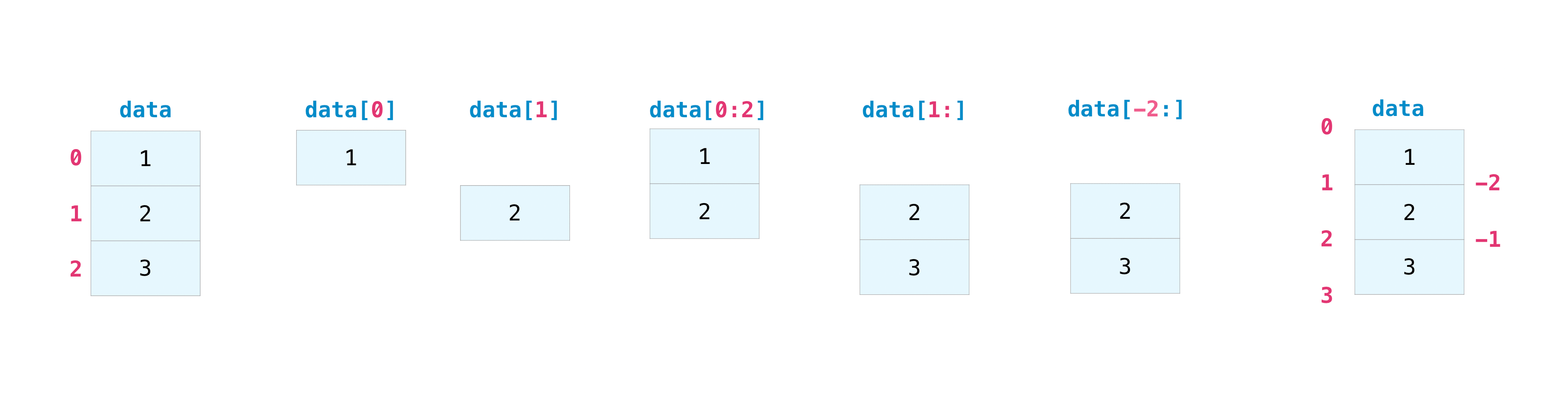
Indexing and slicing

You can index and slice NumPy arrays in the same ways you can slice Python lists.

data = np.array([1, 2, 3])

data[1]

2

data[0:2]

array([1, 2])

data[1:]

array([2, 3])

data[-2:]

array([2, 3])

You can visualize it this way:

You may want to take a section of your array or specific array elements to use in further analysis or additional operations. To do that, you’ll need to subset, slice, and/or index your arrays.

If you want to select values from your array that fulfill certain conditions, it’s straightforward with NumPy.

For example, if you start with this array:

a = np.array([[1 , 2, 3, 4], [5, 6, 7, 8], [9, 10, 11, 12]])

You can easily print all of the values in the array that are less than 5.

print(a[a < 5])

[1 2 3 4]

You can also select, for example, numbers that are equal to or greater than 5, and use that condition to index an array.

five_up = (a >= 5)
print(a[five_up])

[ 5  6  7  8  9 10 11 12]

You can select elements that are divisible by 2:

divisible_by_2 = a[a%2==0]
print(divisible_by_2)

[ 2  4  6  8 10 12]

Or you can select elements that satisfy two conditions using the & and | operators

c = a[(a > 2) & (a < 11)]
print(c)

[ 3  4  5  6  7  8  9 10]

You can also make use of the logical operators & and | in order to return boolean values that specify whether or not the values in an array fulfill a certain condition. This can be useful with arrays that contain names or other categorical values.

five_up = (a > 5) | (a == 5)
print(five_up)

[[False False False False]
 [ True  True  True  True]
 [ True  True  True  True]]

If you want to generate a list of coordinates where the elements exist, you can zip the arrays, iterate over the list of coordinates, and print them. For example:

list_of_coordinates = list(zip(a[0], a[1]))
for coord in list_of_coordinates:
    print(coord)

(1, 5)
(2, 6)
(3, 7)
(4, 8)

Basic array operations

Once you’ve created your arrays, you can start to work with them. Let’s say, for example, that you’ve created two arrays, one called “data” and one called “ones”:

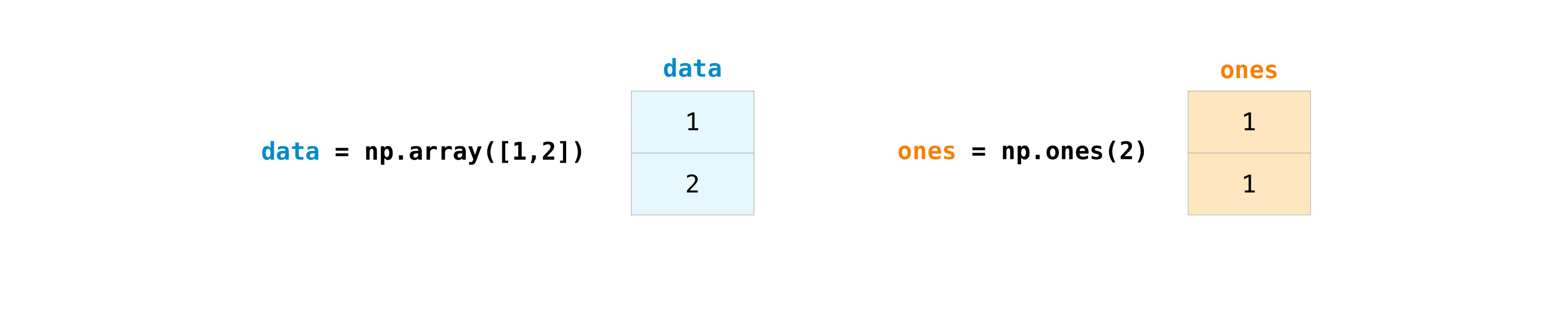
You can add the arrays together with the plus sign.

data = np.array([1, 2])
ones = np.ones(2, dtype=int)
data + ones

array([2, 3])

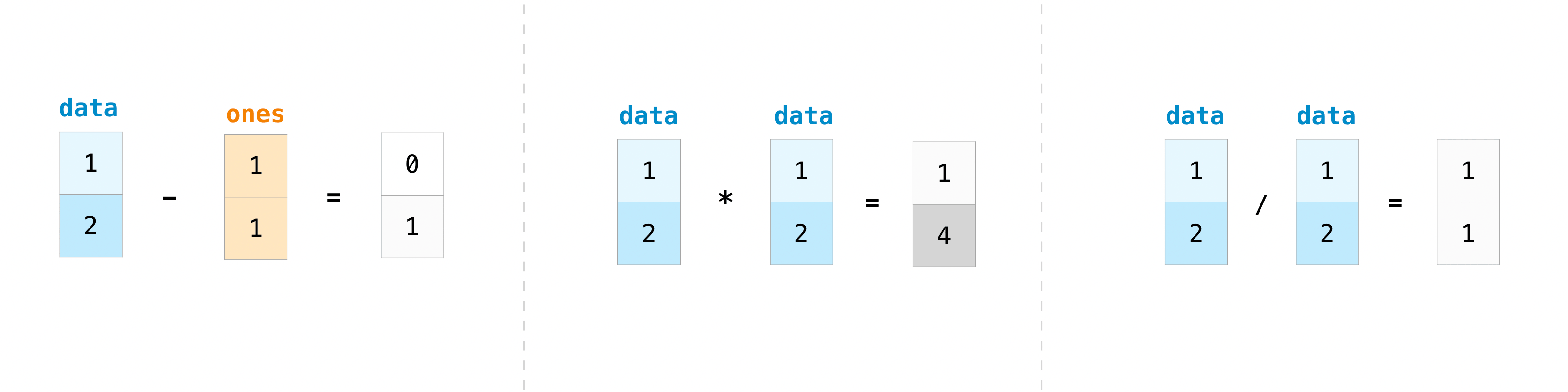
You can, of course, do more than just addition!

data - ones

array([0, 1])

data * data

array([1, 4])

data / data

array([1., 1.])

Basic operations are simple with NumPy. If you want to find the sum of the elements in an array, you’d use sum(). This works for 1D arrays, 2D arrays, and arrays in higher dimensions.

a = np.array([1, 2, 3, 4])
a.sum()

10

To add the rows or the columns in a 2D array, you would specify the axis.

If you start with this array:

b = np.array([[1, 1], [2, 2]])

You can sum over the axis of rows with:

b.sum(axis=0)

array([3, 3])

You can sum over the axis of columns with:

b.sum(axis=1)

array([2, 4])

And you can do other operations like finding the minimum value, maximum value, mean, and more. For example, to find the minimum value in an array, you’d use min():

a.min()

1

To find the maximum value in an array, use max():

a.max()

4

To find the mean of the elements in an array, use mean():

a.mean()

2.5

How to get unique items and counts

You can find the unique elements in an array easily with np.unique.

For example, if you start with this array:

a = np.array([11, 11, 12, 13, 14, 15, 16, 17, 12, 13, 11, 14, 18, 19, 20])

you can use np.unique to print the unique values in your array:

unique_values = np.unique(a)
print(unique_values)

[11 12 13 14 15 16 17 18 19 20]

To get the indices of unique values in a NumPy array (an array of first index positions of unique values in the array), just pass the return_index argument in np.unique() as well as your array.

unique_values, indices_list = np.unique(a, return_index=True)
print(indices_list)

[ 0  2  3  4  5  6  7 12 13 14]

You can pass the return_counts argument in np.unique() along with your array to get the frequency count of unique values in a NumPy array.

unique_values, occurrence_count = np.unique(a, return_counts=True)
print(occurrence_count)

[3 2 2 2 1 1 1 1 1 1]

Generating random numbers

The last topic we’ll cover here is random sampling. The use of random number generation is an important part of the configuration and evaluation of many numerical and machine learning algorithms. Whether you need to randomly initialize weights in an artificial neural network, split data into random sets, or randomly shuffle your dataset, being able to generate random numbers (actually, repeatable pseudo-random numbers) is essential.

Here are some of the most commonly used functions:

• np.random.rand(): generates random numbers between 0 and 1.

• np.random.randn(): generates random numbers from a standard normal distribution (mean 0, standard deviation 1).

• np.random.randint(): generates random integers between a specified range.

• np.random.choice(): randomly selects elements from an array.

• np.random.permutation(): randomly permutes a sequence (e.g., an array).

• np.random.shuffle(): randomly shuffles a sequence in place.

• np.random.choice(): randomly selects elements from an array.

Here’s an example of how to use np.random.rand() to generate an array of random numbers:

# Generate an array of 10 random numbers between 0 and 1
random_numbers = np.random.rand(10)

print(random_numbers)

[0.43173237 0.87249775 0.04039115 0.09135611 0.88631414 0.34073253
 0.49297186 0.96860187 0.39171388 0.21279904]

We output an array of 10 random numbers between 0 and 1.

You can also use the np.random.seed() function to set a seed for the random number generator. This can be useful if you want to generate the same set of random numbers each time you run your code. For example:

# Set the seed for the random number generator
np.random.seed(42)

# Generate an array of 10 random numbers between 0 and 1
random_numbers = np.random.rand(10)

print(random_numbers)

[0.37454012 0.95071431 0.73199394 0.59865848 0.15601864 0.15599452
 0.05808361 0.86617615 0.60111501 0.70807258]

This will generate the same set of 10 random numbers each time you run the code, because the seed for the random number generator has been set to 42. This is important for reproducibility - the ability to produce the same results across different runs.

Let’s do it again (notice how we produce the same set of random numbers):

# Set the seed for the random number generator
np.random.seed(42)

# Generate an array of 10 random numbers between 0 and 1
random_numbers = np.random.rand(10)

print(random_numbers)

[0.37454012 0.95071431 0.73199394 0.59865848 0.15601864 0.15599452
 0.05808361 0.86617615 0.60111501 0.70807258]

Here’s an example of how to use np.random.permutation() to randomly permute an array:

# Create an array of numbers from 1 to 10
numbers = np.arange(1, 11)

# Randomly permute the array
permuted_numbers = np.random.permutation(numbers)

print(permuted_numbers)

[ 9  3  1  7  8 10  4  2  5  6]

This outputs an array of the numbers from 1 to 10, randomly permuted.

You can also use the np.random.choice() function to randomly select elements from an array. Here’s an example that will output an array of 3 random numbers selected from the array.

# Create an array of numbers from 1 to 10
numbers = np.arange(1, 11)

# Randomly select 3 numbers from the array
random_numbers = np.random.choice(numbers, size=3, replace=False)

print(random_numbers)

[2 8 7]

Next steps

This tutorial has covered many of the basics of NumPy that you’ll need to get started with data analysis in Python. If you want to learn more, you can check out the NumPy User Guide or the NumPy Reference.

Try working through on your own. Here are some simple exercises to get you started:

1. Statistical Calculations

Write a Python program that does the following:

• Create a NumPy array containing five random integers between 1 and 1000.

• Calculate and print the following statistics for the array:

• Mean

• Median

• Max

• Min

• Sum

Example output:

Array: [12 27 33 8 41]
Mean: 24.2
Median: 27.0
Standard Deviation: 13.088
Max: 41
Min: 8
Sum: 121

# Insert your code here.

1. Element-wise Operations

Write a Python program that does the following:

• Create two NumPy arrays, array1 and array2, containing five random integers between 1 and 10.

• Perform element-wise addition, subtraction, multiplication, and division between array1 and array2.

• Print the results.

Example output:

Array 1: [5 3 9 7 2]
Array 2: [8 1 6 4 10]
Addition: [13 4 15 11 12]
Subtraction: [-3 2 3 3 -8]
Multiplication: [40 3 54 28 20]
Division: [0.625 3.    1.5   1.75  0.2  ]

# Insert your code here.

1. Indexing and Slicing

Write a Python program that does the following:

• Create a NumPy array containing numbers from 1 to 20.

• Print the element at index 5.

• Print the elements from index 10 to the end.

• Print the elements from index 5 to index 15.

• Print every second element in the array.

Example output:

Array: [1 2 3 4 5 6 7 8 9 10 11 12 13 14 15 16 17 18 19 20]
Element at index 5: 6
Elements from index 10 to the end: [11 12 13 14 15 16 17 18 19 20]
Elements from index 5 to index 15: [6 7 8 9 10 11 12 13 14 15]
Every second element: [1 3 5 7 9 11 13 15 17 19]

# Insert your code here.